Data Driven - Our Blog

The Goal

In this blog post, we will explore the capabilities and workflow for generating, evaluating, and utilizing machine learning (ML) models in BigQuery from Looker. Specifically, we will focus on developing a basic linear regression model to estimate the total number of conversions (purchases) on a website based on the daily sessions and various events such as product views and items added to the cart.

Throughout this blog, we will discuss the general workflow involved in generating ML models, including loading and processing data, performing exploratory data analysis, selecting relevant features, and creating training datasets. We will also cover the selection of the ML model type and its options, as well as using the model for predictions and interpreting the results.

By the end of this blog post, readers will have a solid understanding of how to leverage BigQuery ML and Looker to develop and deploy ML models, enabling them to try it out on their own.

Data Source

A test data model previously loaded in Looker has been used. The Explore used contains relevant information about eCommerce sessions.

General Workflow

Generally, this type of project will include the following steps:

Load data to Bigquery
Clean and process data
Perform EDA (Exploratory Data Analysis)
Select features and create a training dataset
Select ML model type and specify options
Use the model for predictions
Interpret results on a dashboard
Evaluate and improve model performance

In our specific case, steps 1 and 2 have already been completed, as we already have the test data in BigQuery. Therefore, we will proceed to explain the remaining steps.

Perform EDA

Performing exploratory data analysis (EDA) is crucial for understanding and interpreting the data provided, identifying and correcting anomalies that could affect the model's performance, and gaining insights into the underlying patterns and relationships in the data.

This helps make informed decisions about data preprocessing, feature selection, and model development.

In our case, some variables have been detected:

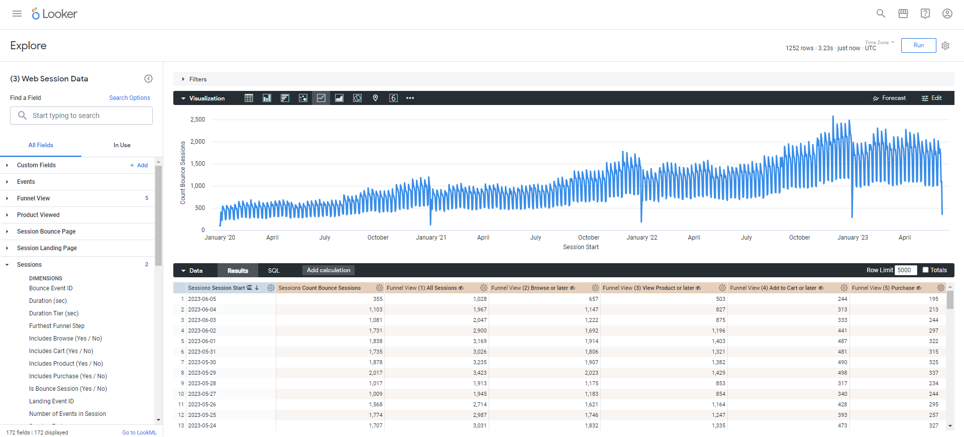
Some weekly patterns in the number of sessions recorded. For example, there is a pronounced drop every December 31.
It's important to note that the data is not up to date, with the last recorded data dated back to 2023-06-05 UTC. This lack of up-to-date data prevents us from building a model that can be constantly be trained with new data, but for the purpose of this walkthrough, we can still implement the model.
We have approximately 3 years of data to work with, which would seem to be sufficient. Keep in mind that there's no general rule regarding the amount of data; typically, the more (relevant) data we have, the more certainty we can derive from the results.

Figure 1 shows the seasonality mentioned above and the available range of data.

Select Features and Create a Training Dataset

Now that we’ve completed EDA, we will develop a regression model to try to estimate the total daily conversions of the site. Based on this, and on the information available in the dataset, the variables that could have the highest correlation with the total conversions were selected.

With this, an NDT was created as shown below:

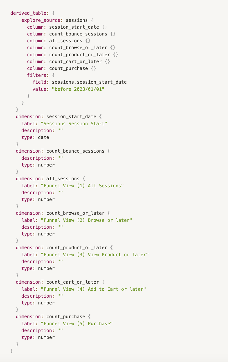
count_purchase will be our target variable. This variable indicates the number of sales that occurred on the page. It is important that we can predict this value as it will directly impact our revenue forecast. The variables we will use as predictors of the target are the number of other events (how many sessions there were, how many of those sessions added products to the cart, how many viewed a product, how many sessions ended after the first page view, etc). At first glance, we might assume that the more sessions the site has, the more sales we might expect. The same goes for the more of those sessions that add a product to the cart, as it denotes an intention to buy. However, the model will be responsible for indicating whether our assumptions are correct.

Note that we have included a filter to use only the sessions up to 2022-12-31 to create and train the model. The 2023 data will be used as a validation set to make further predictions and interpret the results. The validation set will be used to evaluate how good our model is at predicting the target variable.

With this, we make the model predict the target variable for a dataset that it has not yet "seen" (since we did not use it to train it).

Then, we will compare its predictions with the actual value of the target variable, which we already know, and see how good its predictions were. You can learn more about training, testing and validation sets in this link.

In our case, all records from 2023 will be our validation set. However, in datasets that are constantly updated, it would be advisable to generate relative time filters, so that the model can be constantly updated and retrained as new data becomes available.

NOTE: BigQuery ML automatically splits your input data into a training set and a holdout set to avoid overfitting the model. However, in this demonstration it has been decided to manually create separate datasets for easier interpretation of the results. You can edit the way in which a model stops the dataset with the parameter DATA_SPLIT_METHOD.

Select ML Model Type and Specify Options

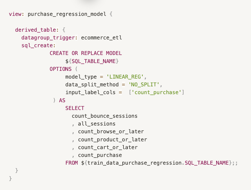
Now we will create a new view to define the model. Within the "OPTIONS" parameter, a multitude of options are defined and parameterized depending on the model chosen. All available options for linear regression models are available in the official documentation. General information on all available model types can be found at the following link.

Some things to consider:

The command sql_create replaces the CREATE OR REPLACE statement in BQML and tells Looker to execute the command as is, without Looker’s usual error checking.
This command also requires the creation of a persistent derived table (PDT), and when used in tandem with a datagroup trigger becomes a powerful way to control how long the results of this model should be saved before being rebuilt with new data.
We use data_split_method to prevent BigQuery from automatically separating the input data into train and test, since we have created a separate dataset for prediction and evaluation.

Use Model For Predictions

Next, we’ll create an identical view which is exactly the same as the training set, except that we change the date filter to take data from 2023.

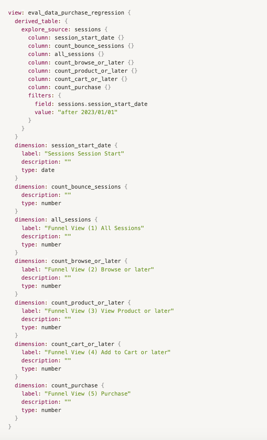
Then, we’ll create a new dataset on which the predictions will be made:

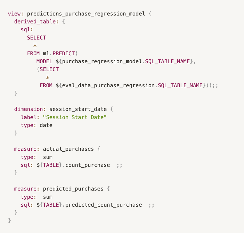
ml.PREDICT generates the prediction and creates a new variable called predicted_<label_column_name>. For more information on the ml.PREDICT function, please click on the following link.

Explaining the ml.EXLAIN_PREDICT Function

Instead of ml.PREDICT we can use the function ml.EXPLAIN_PREDICT, which gives us additional information to understand how the model works. The additional options will depend on the type of model developed. You can also learn more about linear regression models in this link.
For example, in the case of linear regression, the function can give us the top_feature_attributions data, which tells us how each variable of the model influences the final prediction.
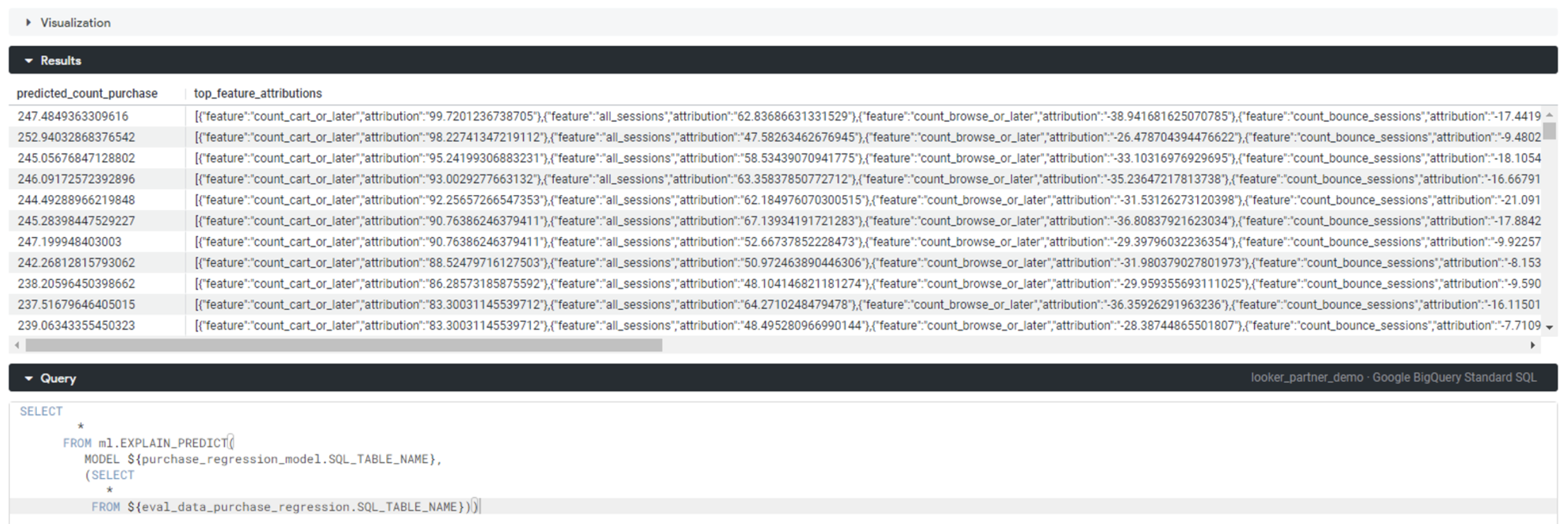
The image below shows the use of EXPLAIN_PREDICT. In our case, we can highlight the following points:
- The model stores the predictions in a new variable called "predicted_[target variable]". So in our case, the value in "predicted_count_purchase" indicates the amount of sales the model has estimated there will be on a given day.
- We must then compare this value with the actual value of sales on those dates to evaluate how well our model has performed.
- For linear regression models (such as ours), top_feature_attributions orders the variables from most to least influential. This means that the first variable we see in the list is the one that has had the most influence on the final prediction, which is seen in the highest value of "attribution".
- The positive or negative sign of "attribution" indicates whether the relationship between that variable and the target is directly or inversely proportional. A negative number indicates that if this variable increases, our target will decrease. For example, the number of Bounce Sessions has an inversely proportional relationship to the amount of purchases (which makes sense theoretically).

Interpreting Results + Visualization

Evaluate Model

For this we can make use of the ml.EVALUATE function. This returns a single row containing metrics applicable to the type of model specified.

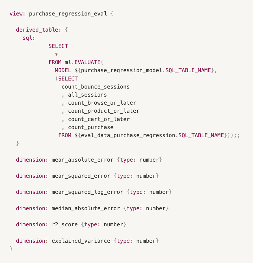
More information on the metrics returned for each model can be found in the following link. General information on how to perform a model evaluation can be found in the following link.

Visualize The Results

We can generate Explores and Looks with the dimensions and metrics generated, for a better interpretation of the results. Here's an example dashboard with the results of the predictions performed.

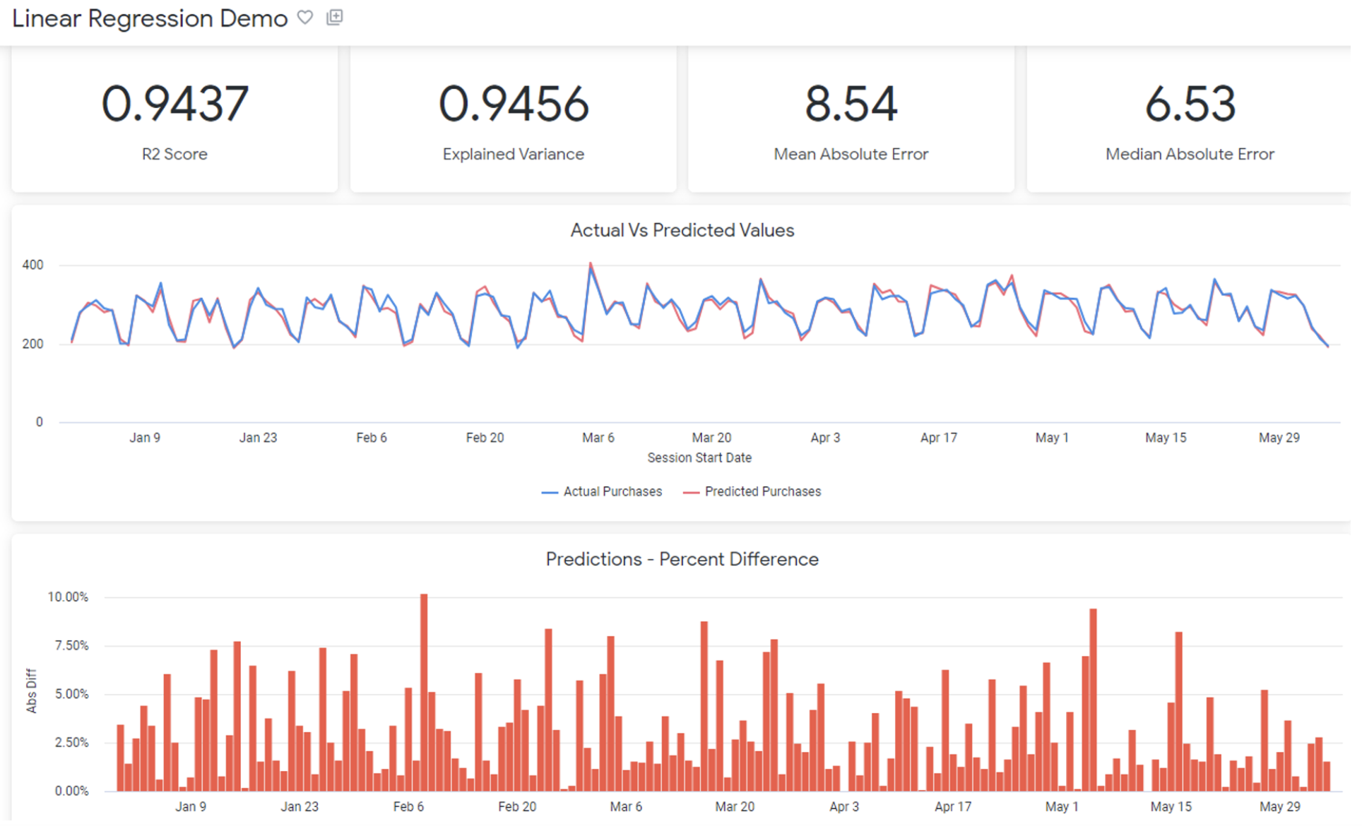
The metrics in the dashboard show:

R2 Score: this is a measure that provides information about the “goodness of fit." In the context of regression it is a statistical measure of how well the regression line approximates the actual data.
Explained Variance: measures the discrepancy between a model and actual data. In other words, it’s the part of the model’s total variance that is explained by factors that are actually present. Higher percentages of explained variance indicates a stronger strength of association. It also means that you make better predictions.
Mean Absolute Error: is the average variance between the actual values of the data set and the projected values predicted by our model.
Median Absolute Error: same as above, but we take the median of the errors instead of the average.

What Does This Mean about Our Model?

It can be observed that, in general terms, the predictions have been relatively accurate. The prediction curve was able to reflect the seasonality observed in the actual data. The R2 is 0.9437. The closer to 1 generally implies that the model adequately represents the observed data. However, care must be taken not to cause overfitting.

Overfitting is a concept in data science, which occurs when a statistical model fits exactly against its training data.

When this happens, the algorithm unfortunately cannot perform accurately against unseen data, defeating its purpose.

Overfitting the model generally takes the form of making an overly complex model to explain data under study. In reality, the data often has some degree of error or random noise within it.

Thus, attempting to make the model conform too closely to slightly inaccurate data can infect the model with substantial errors and reduce its predictive power. You can learn more about overfitting by following this link.

Tips And Best Practices

Here are some practices that might help you to better develop models with BigQuery ML and Looker.

Create a separate folder within Looker views to store files related to your model.
As a general rule, it is advisable to separate the views related to the creation of train and test datasets, model development, evaluation and prediction generation into different files.
Declare explicitly the fields to be used to train the model. Although it is supported by BigQuery, using SELECT * may cause us to erroneously incorporate some unnecessary variables, affecting the performance of the model.
When possible, use relative date filters to create the data sets with which you will train and evaluate the model. This would allow the model to be constantly trained with updated information and kept up to date. For example, instead of training the model with data from the year 2023, you could do so with a "last 12 months" filter.
While BigQuery can automatically separate the dataset into train, test and/or evaluation, it may be a good idea to perform this separation manually in some cases, in order to have a better control of each dataset separately and to be able to evaluate the results in more detail.
Another option is to create a specific column to separate the dataset into train and test and use other features of the CREATE MODEL function such as DATA_SPLIT_COL and DATA_SPLIT_EVAL_FRACTION. You can find more information about this in the following link.
You can use the ml.TRANSFORM function in case you need to transform the data before it can be used by the model. You can find more information about transformations in the following link.
Some models can be used with hyper parameter tuning. You can find more information in the following link.

Conclusion

Hopefully this blog provides you with a comprehensive overview of the capabilities and workflow for generating, evaluating, and utilizing machine learning (ML) models in BigQuery from Looker. Just remember that to train an efficient model, you’ll need lots of well organized data.

If you want to learn more about how to leverage Google Cloud Platform for your business and get the most out of it, subscribe to our newsletter or reach out to us with any questions. Happy modeling!